
Using MySQL with R
- Benefits of a Relational Database
- Connecting to MySQL and reading + writing data from R
- Simple analysis using the tables from MySQL
If you’re an R programmer, then you’ve probably crashed your R session a few times when trying to read datasets of over 2GB+. It can get a little frustrating when all you want to do is harness the true power behind R through building statistical models on these large datasets, and your session crashes with a window stating “R SESSION ABORTED”. Since R executes code in-memory, which is the computers available RAM, you will encounter failures when reading datasets larger than the available memory. Also, once you have enough data frames stored, then your R session can become extremely slow and affect your work severely. One of my classes at Pace University showed me the value in storing your larger datasets in a MySQL database, and I decided to learn how to stream these datasets in R, so we do not have to store the larger datasets in-memory. This post will briefly discuss a few advantages of using a database to store your data and run through a basic example of using R to transfer data to and from MySQL. I will assume you already have access to a MySQL database.
#Relational Database vs In Memory
Relational databases like MySQL, organize data into tables (spreadsheet format) and can link values in tables to each other (hence “relational”). These relationships are columns that are stored as “unique” & “foreign” key values. Generally speaking, they are better at handling large datasets and are more efficient at storing and accessing data than CSVs due to compression and indexing rules. The data is stored on-disk with MySQL, until it is called through a query, which is different from the in-memory approach R uses for data.frames, matrices, tibbles, vectors, etc. When reading data stored in a file or data.frame in R, the data must all fit in the current available RAM memory.
#The Data
We will use the Chicago Parking Ticket dataset from here which contains 2.07GB 28,272,580 rows containing details on all parking and vehicle compliance tickets issued in Chicago from Jan. 1, 2007 to May 14, 2018, from the Chicago Department of Finance. This isn’t necessarily a “large” dataset, but I believe it’s a large enough size to notice a difference in the performance. First, I am going to read a smaller portion of the data to get an idea of the data types inside the table.
#Fread to quickly load into R to get a sense of what your data looks like.
test.csv <- data.table::fread("/usr/local/mysql-8.0.15-macos10.14-x86_64/data/parking_tickets.csv", nrows = 1000000)

#View
str(test.csv)
## Classes 'data.table' and 'data.frame': 1000000 obs. of 23 variables:
## $ ticket_number :integer64 51551278 51491256 50433524 51430906 51507779 51260468 51501733 51260469 ...
## $ issue_date : chr "2007-01-01 00:00:00" "2007-01-01 00:00:00" "2007-01-01 00:01:00" "2007-01-01 00:01:00" ...
## $ violation_location : chr "6014 W 64TH ST" "530 N MICHIGAN" "4001 N LONG" "303 E WACKER" ...
## $ license_plate_number : chr "90ad622c3274c9bdc9d8c812b79a01d0aaf7479f2bd7431f8935baa4048d0c86" "bce4dc26b2c96965380cb2b838cdbb95632b7b5716061255c7ed9aa52b17163c" "44641e828f4d894c883c07c566063c2d99d08f2c03b3d41682d6d8201a0939bd" "eee50ca0d9be2debd0e7d45bad05b8674a6cf5b892230f54cf1923e36990ada9" ...
## $ license_plate_state : chr "IL" "IL" "IL" "IL" ...
## $ license_plate_type : chr "PAS" "PAS" "PAS" "PAS" ...
## $ zipcode : chr "60638" "606343801" "60148" "60601" ...
## $ violation_code : chr "0976160F" "0964150B" "0976160F" "0964110A" ...
## $ violation_description: chr "EXPIRED PLATES OR TEMPORARY REGISTRATION" "PARKING/STANDING PROHIBITED ANYTIME" "EXPIRED PLATES OR TEMPORARY REGISTRATION" "DOUBLE PARKING OR STANDING" ...
## $ unit : chr "8" "18" "16" "152" ...
## $ unit_description : chr "CPD" "CPD" "CPD" "CPD" ...
## $ vehicle_make : chr "CHEV" "CHRY" "BUIC" "NISS" ...
## $ fine_level1_amount : int 50 50 50 100 25 50 100 50 120 50 ...
## $ fine_level2_amount : int 100 100 100 200 50 100 200 100 240 100 ...
## $ current_amount_due : num 0 50 0 0 0 50 244 0 0 0 ...
## $ total_payments : num 100 0 50 100 50 0 0 50 240 100 ...
## $ ticket_queue : chr "Paid" "Define" "Paid" "Paid" ...
## $ ticket_queue_date : chr "2007-05-21 00:00:00" "2007-01-22 00:00:00" "2007-01-31 00:00:00" "2007-03-08 00:00:00" ...
## $ notice_level : chr "SEIZ" "" "VIOL" "DETR" ...
## $ hearing_disposition : chr "" "" "" "Liable" ...
## $ notice_number :integer64 5048648030 0 5079875240 5023379950 5079891400 0 5038039180 5052314130 ...
## $ officer : chr "15227" "18320" "3207" "19410" ...
## $ address : chr "6000 w 64th st, chicago, il" "500 n michigan, chicago, il" "4000 n long, chicago, il" "300 e wacker, chicago, il" ...
## - attr(*, ".internal.selfref")=<externalptr>head(test.csv)## ticket_number issue_date violation_location
## 1: 51551278 2007-01-01 00:00:00 6014 W 64TH ST
## 2: 51491256 2007-01-01 00:00:00 530 N MICHIGAN
## 3: 50433524 2007-01-01 00:01:00 4001 N LONG
## 4: 51430906 2007-01-01 00:01:00 303 E WACKER
## 5: 51507779 2007-01-01 00:01:00 7 E 41ST ST
## 6: 51260468 2007-01-01 00:03:00 1039 W LELAND
## license_plate_number
## 1: 90ad622c3274c9bdc9d8c812b79a01d0aaf7479f2bd7431f8935baa4048d0c86
## 2: bce4dc26b2c96965380cb2b838cdbb95632b7b5716061255c7ed9aa52b17163c
## 3: 44641e828f4d894c883c07c566063c2d99d08f2c03b3d41682d6d8201a0939bd
## 4: eee50ca0d9be2debd0e7d45bad05b8674a6cf5b892230f54cf1923e36990ada9
## 5: 244116ca3eed4235b1f61f6d753d8c688be2a48c9fdd976fa4c729c6f90f3d76
## 6: b167d28412271c62a8e30cbb5396ffb97f12c08382f9a6f46be4e1c8bb02f444
## license_plate_state license_plate_type zipcode violation_code
## 1: IL PAS 60638 0976160F
## 2: IL PAS 606343801 0964150B
## 3: IL PAS 60148 0976160F
## 4: IL PAS 60601 0964110A
## 5: IL PAS 605053013 0976220B
## 6: IL TMP 60632 0964150B
## violation_description unit unit_description
## 1: EXPIRED PLATES OR TEMPORARY REGISTRATION 8 CPD
## 2: PARKING/STANDING PROHIBITED ANYTIME 18 CPD
## 3: EXPIRED PLATES OR TEMPORARY REGISTRATION 16 CPD
## 4: DOUBLE PARKING OR STANDING 152 CPD
## 5: SMOKED/TINTED WINDOWS PARKED/STANDING 2 CPD
## 6: PARKING/STANDING PROHIBITED ANYTIME 23 CPD
## vehicle_make fine_level1_amount fine_level2_amount current_amount_due
## 1: CHEV 50 100 0
## 2: CHRY 50 100 50
## 3: BUIC 50 100 0
## 4: NISS 100 200 0
## 5: INFI 25 50 0
## 6: BUIC 50 100 50
## total_payments ticket_queue ticket_queue_date notice_level
## 1: 100 Paid 2007-05-21 00:00:00 SEIZ
## 2: 0 Define 2007-01-22 00:00:00
## 3: 50 Paid 2007-01-31 00:00:00 VIOL
## 4: 100 Paid 2007-03-08 00:00:00 DETR
## 5: 50 Paid 2007-08-29 00:00:00 SEIZ
## 6: 0 Define 2007-01-04 00:00:00
## hearing_disposition notice_number officer address
## 1: 5048648030 15227 6000 w 64th st, chicago, il
## 2: 0 18320 500 n michigan, chicago, il
## 3: 5079875240 3207 4000 n long, chicago, il
## 4: Liable 5023379950 19410 300 e wacker, chicago, il
## 5: 5079891400 66396 7 e 41st st, chicago, il
## 6: 0 3307 1000 w leland, chicago, ilGreat, so it looks like our data is mixed between integers, numeric, and character types. We can also see some missing values in some column like “hearing_disposition”. Now its time to insert some of this data into MySQL.
#Connecting to MySQL from R When connecting to any database or connection that requires passwords, it is always highly recommended to store these passwords in your local environment for security reasons. This is especially the case when sharing your code to others or via the internet. Using MariaDB() as the DBI, you need to enter the “user” name, “password” value, “dbname” where your tables are stored, and the “local host”.
#Load RMariaDB if it is not loaded already
if(!"RMariaDB" %in% (.packages())){require(RMariaDB)}

#Connecting to MySQL DB
stuffDB <- dbConnect(MariaDB(), user = "root", password = Sys.getenv("MYSQL_PASSWORD"), dbname = "my_db", host = "localhost")

#List tables in DB
dbListTables(stuffDB)
If connected succesfully, you should see the names of your tables when “dbListTables” is called.
#Creating tables in MySQL from R
Since I want to load the data into MySQL, I need to first create the table that reflects the same columns as the CSV and ensure the data type columns are set correctly. We can see the data types for each column from our earlier “str()” call. See below on how to create a query variable containing SQL syntax.
query<-"CREATE TABLE parking_tickets_chicago (
  ticket_number TEXT,
  issue_date TEXT,
  violation_location  TEXT,
  license_plate_number TEXT,
  license_plate_state TEXT,
  license_plate_type TEXT,
  zipcode TEXT,
  violation_code TEXT,
  violation_description TEXT,
  unit INT,
  unit_description TEXT,
  vehicle_make TEXT,
  fine_level1_amount INT,
  fine_level2_amount INT,
  current_amount_due INT,
  total_payments INT,
  ticket_queue TEXT,
  ticket_queue_date TEXT,
  notice_level TEXT,
  hearing_disposition TEXT,
  notice_number TEXT,
  officer TEXT,
  address TEXT);"


#Send the query to MySQL for execution
results <- dbSendQuery(stuffDB, query)
dbClearResult(results)
#Inserting the data
Now that we have created the table correctly, we can begin inserting the data into the MySQL table directly from R. First we will use a small example before inserting all 28 million rows.
query <- "INSERT INTO parking_tickets_chicago(ticket_number,issue_date,violation_location,license_plate_number,license_plate_state,license_plate_type,zipcode,violation_code,violation_description,unit,unit_description,vehicle_make,fine_level1_amount,fine_level2_amount,current_amount_due,total_payments,ticket_queue,ticket_queue_date,notice_level,hearing_disposition,notice_number,officer,address)
VALUES(51636768,'2007-01-12 10:34:00','1450 N THORNDALE','fc4a98382378c750027d71138b4cbf3237216a6452ec9c3b8c3533f0c1c20d02','IL','TRK',605152677,'0976160F','EXPIRED PLATES OR TEMPORARY REGISTRATION',24,'CPD','TOYT',50,100,0,50,'Paid','2007-01-30 00:00:00','','',0,17482,'1400 n thorndale, chicago, il');"


#Sending the query to MySQL for execution and getting the result.
results <- dbSendQuery(stuffDB, query)


#Checking if it was added correctly
dbReadTable(stuffDB,"parking_tickets_chicago")
So far so good!! We have connected to our database, created a table, inserted data into our new table and check the results. Now let’s do the entire dataset so we can illustrate the value and efficiency of integrating MySQL & R!
Reading all data - Chunk Wise
For any large datasets, I like to use the “read.table” function and create a open connection to the file using file(open=“r”). This way, we can read or write the data chunkwise, instead of all at once in one big operation.
#Create index and select a chunksize
index <- 0
chunkSize <- 100000

#Create column name vector
col_names <- c("ticket_number", "issue_date", "violation_location", "license_plate_number", "license_plate_state", "license_plate_type", "zipcode", "violation_code", "violation_description", "unit", "unit_description", "vehicle_make", "fine_level1_amount", "fine_level2_amount", "current_amount_due", "total_payments", "ticket_queue", "ticket_queue_date", "notice_level", "hearing_disposition", "notice_number", "officer", "address")


#Open the file connection
con <- file(description="/usr/local/mysql-8.0.15-macos10.14-x86_64/data/parking_tickets.csv",open="r")

#Read the data chunkWise
dataChunk <- read.table(con, nrows=chunkSize, header=F, fill=TRUE, sep=",", quote = '"', col.names = col_names)

#Write & append the tables chunkWise
dbWriteTable(stuffDB, value = dataChunk, row.names = FALSE, name = "parking_tickets_chicago", append = TRUE)


#Repeat for each dataChunk
while (nrow(dataChunk) > 0) {
  index <- index + 1
  print(paste('Processing rows:', index * chunkSize))

  dataChunk <- read.table(con, nrows=chunkSize, skip=0, header=FALSE, fill = TRUE, sep=",", col.names = col_names)

  dbWriteTable(stuffDB, value = dataChunk, row.names = FALSE, name = "parking_tickets_chicago", append = TRUE)
}

#Close the open file connection
close(con)
Let me explain the above process step by step so it easier to understand.
Step 1. Create our index, chunk size, col_names, and file connection variables. We are choosing a chunk size of 100k. This means that each index is 100,000 rows of the data frame, so index 1 is 1-100k, index 2 is 100k-200k, index 3 is 200-300k, and keeps increasing until all of our rows have been read chunkwise. This allows you to run arithmetic operations on datasets too large to read in memory.
Step 2. Once we set these, we can create our “dataChunk” using our variables as the values for read.table arguments.
Step 3. Each dataChunk is sent to our newly created table in MySQL and will be appended to our newly created table since we set “append=TRUE” in our dbWriteTable() call.
Step 4. Repeat this until all the data has been read through each chunk and our while statement is satisfied.
Now let us run a simple SQL and R query to interact with the MySQL database. The “dplyr” package makes it possible for us to use R code instead of SQL, to extract and manipulate from the database because it converts the R query to SQL before it’s sent to the DB.
#MySQL query
Let us do a very simple query to count the issued tickets by month. We can create a graph to visualize which month had the most tickets issued.
query <- "SELECT monthname(issue_date) as month, year(issue_date) as year, count(ticket_number) as number
FROM my_db.parking_tickets_chicago
GROUP BY month,year
HAVING month is not null AND year is not null;"


results <- dbSendQuery(stuffDB, query)
db_results <- dbFetch(results)
dbClearResult(results)

#Filter out any results that could possibly be an error due to the data-entry mistake for date
db_results <- db_results %>% filter(number != 1) %>% mutate(month = factor(month,levels = month.name), year = as.integer(year), number = as.numeric(number)) %>% arrange(year)


#Preview of our results
head(db_results)

#Plot
ggplot(db_results, aes(factor(month,levels = month.name),number)) +
  geom_bar(stat="identity", aes(fill = year)) +
  labs(
    title = "Boxplot",
    subtitle = "Count of Tickets by Month",
    x="Month",
    y="Occurences"
    ) +
  scale_y_continuous(labels = scales::comma) +
  scale_fill_continuous("Year", breaks=c(2008:2018), labels = c(2008:2018), type = "viridis") +
  theme_dark() +
theme(axis.text.x = element_text(angle=50, vjust=0.65)) 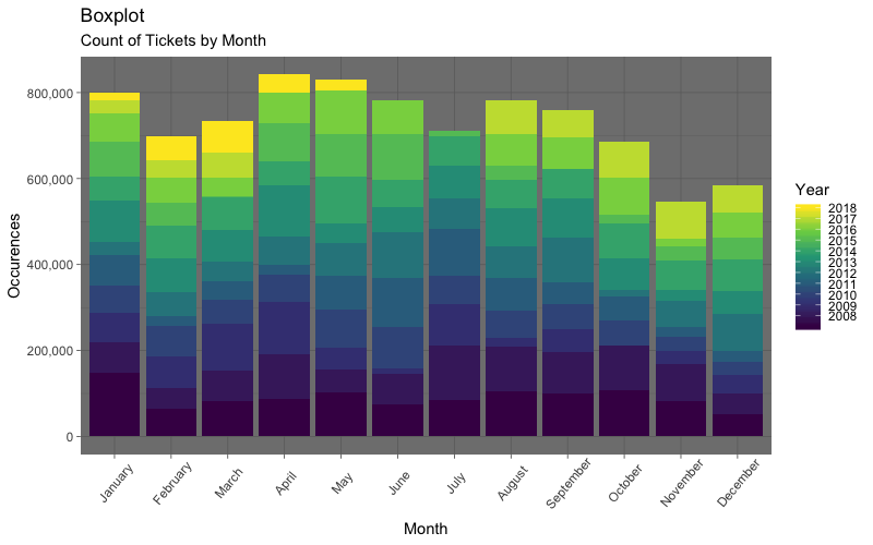
R query using Dplyr
We can even do the same thing but all in R without having to use any SQL. This is beneficial for the users who don’t use SQL and also makes it easier to share. Although, the time difference in performance is noticeable between these two approaches. I believe it’s best to just use SQL syntax since it seems more efficient, but I will review this using R syntax below.
library(dplyr)
library(lubridate)

#Reads part of the dataframe in our DB so it does not store it all in memory
search_db <- tbl(stuffDB, "parking_tickets_chicago")

#R syntax using dplyr
search_db <- search_db %>%
  select(issue_date, ticket_number) %>%
  mutate(month = month(issue_date), year = year(issue_date), number = ticket_number) %>%
  filter(month != "" & year != "") %>%
  group_by(month, year) %>% select(month,year,number)


print(search_db)


#Show how dplyr converts the R code to SQL behind the scenes.
show_query(search_db)

#Close connection
dbDisconnect(stuffDB)
#Wrapping it up
Not only did we use SQL syntax to read/write data to our MySQL database from R, but we also used R syntax to do it as well! With the help of the “dplyr” package, you can use only R syntax to wrangle data stored in your MySQL database. Clearly, using MySQL with R will not only prevent unnecessary data clogging the memory but also saves time since the chunkWise approach cuts the writing time down significantly. If you’re an R programmer who runs into large datasets, even if it’s just occasionally, then I highly suggest you look into using MySQL or any other relational databases with R.
