
Conference Call Text Mining and Sentiment Analysis
- Executives are very careful with the language they use during a conference call
- Using sentiment scores to validate future / long-term goals
- Checking for negation words that can affect score
- Key takeaways from this analysis
Do you ever notice when our president sends out a tweet and the markets spike/drop almost instantly, or within seconds of news going public, millions of shares are being traded based off what was said or done? Are investors staring at twitter 24/7 ready to hit buy or sell? The answer, of course, is no, but algorithms programmed with NLP (natural language processing) scripts are. Sentiment analysis from tweets, social media postings, press releases, surveys, reviews, transcripts and many more occur millions of times every day. Even when you send your resume in to apply for a job, most likely your resume is being read through an ATS system which analyzes the text to find matching keywords. I’ve had this earnings sentiment script locked away in my useful financial scripts vault, and after reading a Stanford research paper titled “Forecasting Returns Using Earnings Call Transcripts” it inspired me to build upon my current script and create a post about earnings call sentiment.
I’ll create part 1 and 2 for this subject because while attempting to cover all the basics, part 1 resulted in a somewhat lengthy post. After cleaning the text, I will use the simple method of word frequency analysis, incorporate a variety of lexicons for sentiment analysis to arrive at overall sentiment scores, adjust the lexicons to fit our criteria, search for possible negation words, and use network graphs to visualize relationships between the text. In part 1, I will review the basics of sentiment analysis in R while in part 2 I will build a model to help us predict if the earnings call warrants a buy for the stock.
Getting the Data
First, I want to create an empty data frame that will hold the results of each lexicon. After, I will web scrape the transcript from seeking alpha and clean any empty spaces from the data. Then, I can begin extracting the key text using Regular Expression (REGEX) and putting it together into seperate data frames. Regular expression is a pattern matching tool that makes up a sequence of symbols to search and extract pattern in the text.
#Create empty sentiment dataframe that we will build for each lexicon
sentiment_df <- tibble(Ticker=NA,Earnings_date=NA,Positive=NA,Negative=NA,Total_words=NA,Score=NA,Sentiment=NA, Lexicon=NA)

#Company Info
company_name <- "salesforce"
ticker <- "CRM"

#Transcript URLs
q1 <- "https://seekingalpha.com/article/4177957-salesforce-com-inc-crm-ceo-marc-benioff-q1-2019-results-earnings-call-transcript?part=single"


q4 <- "https://seekingalpha.com/article/4246320-salesforce-com-inc-crm-ceo-marc-benioff-q4-2019-results-earnings-call-transcript?part=single"


#Requesting html
html1 <- read_html(q4)

#Reading the body of the html, and converting it to a readable text format
transcript_text <- html_text(html_nodes(html1, "#a-body"))

#Seperating the text by new line characters in html code
transcript_text <- strsplit(transcript_text, "\n") %>% unlist()


#Remove empty lines
transcript_text <- transcript_text[!stri_isempty(transcript_text)]

#Getting the earnings date
earnings_date <- html_text(html_nodes(html1, "time")) %>% paste0(collapse = "")
Regular Expression
If new to REGEX, it can look like nonsense but it is very powerful to sort through and filter textual data. As an example, look at the REGEX code below that I found off google that searches for simple email addresses;
[a-zA-Z0-9_.+-]+@[a-zA-Z0-9_-]+\.[a-zA-Z0-9_.-]+
I want to extract the names of executives and analysts in the transcript. I can do this by matching the text to a common format found in transcripts. The transcripts start out by listing the conference call participants, and the lines containing the names always use either “-” or “–” as separators for NAME - TITLE.
TIP: If REGEX is too daunting for you, then R provides a package called “Rebus” that makes using REGEX as easy as using words to represent patterns. For example, the first the block of code below, and notice how it uses words like “upper, one_or_more, SPC, WRD, capture” instead of the REGEX syntax “[[:upper:]][\w]+”.
Splitting the text into sections for analysis
#Create pattern to grab relevant names such as Analyst and Executives.


#Using Rebus
pattern1 <- capture(upper() %R% one_or_more(WRD) %R% SPC %R%
  upper() %R% one_or_more(WRD)) %R% " - " %R% capture(one_or_more(WRD) %R%
  optional(char_class("- ,")) %R% zero_or_more(WRD %R% SPC %R% WRD %R% "-" %R% WRD))


#Give the names all common seperators
transcript_text <- gsub("–","-",transcript_text)


#REGEX pattern to search for the starting index containing executive names. Finds something like "Mark Benioff - CEO"
idx_e <- min(which(str_detect(transcript_text, "[[:upper:]][\\w]+ -")))


#Dropping everything before the start of Executive names, and resetting the index back to 1
transcript_text <- transcript_text[idx_e:length(transcript_text)]
idx_e <- 1


#Repeating to find the starting index for the analyst names
idx_a <- min(which(!str_detect(transcript_text, "[[:upper:]][\\w]+ -")))


#Executive names will start from the starting index, idx_e, to 1 row before the analysts starting index, idx_a. We will use the Rebus pattern we created to extract all names from our resulting vectors
exec <- transcript_text[idx_e:(idx_a-1)]
exec <- str_match(exec, pattern1)
exec <- exec[1:nrow(exec),2]


#Repeat for the Analyst names. The ending index for the analyst names is the row before the opening remarks
idx_o <- min(which(!str_detect(transcript_text, "[[:upper:]][\\w]+ -"))[-1]) - 1
analyst <- transcript_text[(idx_a+1):idx_o]
analyst <- str_match(analyst, pattern1)
analyst <- analyst[1:nrow(analyst),2]


#Save just the transcript text. Skip straight to the operators opening remarks
transcript_text <- transcript_text[(idx_o +1) : length(transcript_text)]


#Splitting up the call between management on the conf_call and the Q&A session

#Start with Conf_call section and find the start of the Q&A
idx_c <- min(which(str_detect(transcript_text, paste(exec,collapse = "$|"))))
idx_q <- which(str_detect(transcript_text, "Question-and-Answer")) - 1
conf_call <- transcript_text[idx_c:idx_q]


#Now for the QNA section
idx_q <- which(str_detect(transcript_text, "Question-and-Answer")) + 1
qna <- transcript_text[idx_q:length(transcript_text)]


#Get locations of the names so we can label the text in order
conf_location_exec <- str_which(conf_call, paste(exec,collapse = "$|^"))
exec_names_conf <- conf_call[conf_location_exec]


#Get locations of the names so we can label the text in order
qna_location_analysts <- str_which(qna, paste(analyst, collapse = "$|^"))
qna_location_exec <- str_which(qna, paste(exec, collapse = "$|^"))


#Create tibble then combine and arrange by row id to keep the correct order
analyst_names_qna <- tibble(name = qna[qna_location_analysts], id = qna_location_analysts)
exec_names_qna <- tibble(name = qna[qna_location_exec], id = qna_location_exec)
all_names_qna <- bind_rows(analyst_names_qna, exec_names_qna) %>% arrange(id)
After extracting the information I need, the earnings transcript is then broken up into two data frames. The first data frame is the first half of the call when the management announces results; then the second data frame is the question and answer session of the call which both are labeled by who is speaking. The first data frame is “conf_call_df” and the second is “qna_full”. This will help give additional visualization once we start getting sentiment scores. Take a look at the first three interactions from the qna_full data frame below.
The first three interactions from the qna_full data frame
kableExtra::kable(head(qna_full,3)) %>% kableExtra::kable_styling()| names | text |
|---|---|
| Phil Winslow | Congrats on a great start to the year and a particular shout out to Hawkins for the awesome 606 data historically, super helpful. A question for Marc B on MuleSoft, I mean obviously, nobody knows CRM data better than salesforce.com. But wondering if you could talk about Einstein and MuleSoft, and that in the AI context, because obviously you’re delivering already 2 billion predictions? How do you think MuleSoft, or how do you see MuleSoft, augmenting that? And what kind of uptick you think you’ll see their insight customers? |
| Marc Benioff | Well, as we go deeper into our vision with so many of our customers, the key thing that we are focused on is their single view of their customer. We just talked about so many of our key wins in the quarter. I mean, it could be carrying with their reprocessing incredible brands like Gucci, or Bottega or Yves Saint Laurent, the UFDA and their relationship with their farmers and ranchers, it could be the work that we’re doing with the [Align] [ph], giving their orthodontist the ability to connect with their consumers in a whole new way, or it could be the incredible work that you’re seeing with Adidas.In each and every case, they’re working to understand and have a 360 degree view of their customer. And the power of that is really augmented by our suite of CRM applications that do that for them. Things like our sales, commerce, service, communities, analytics, our core platform, collaboration, marketing and exactly what you said, by adding integration in that, it helps us bring in data from multiple public clouds, because many of our customers are now using multiple public clouds and/or they might be, let’s say for example, the healthcare company seeking data from the healthcare system itself like an insurance system, or maybe some other type of key databank associated with the healthcare industry, integration is mission-critical for our customers to gain that 360 degree view of their customer.Now, we’ve always known that at Salesforce, that’s why we built up an open system. And that’s why we’ve had an application program interface. That’s why we’ve had an AppExchange. That’s why we focused on ISVs and had relationships with companies like MuleSoft. But it has become more important for our customers to be able to have and rely on an integration cloud. This idea of deeply embedded inside our products, they can rely on this technology to be able to integrate all the key data so they can build that single view of the customer.And we have Bret Taylor here who is our President and Chief Product Officer. And Bret, do you want to just touch on that and your – I know you’ve been traveling the country and talking to hundreds of our customers about their vision for integration. Can you tap that for us? |
| Bret Taylor | Yes, sure. When we talk to our customers, they talk about three main priorities as it relates to integration. They want to create customer experiences that transcend individual customer touch points. They want to integrate sales, service, and marketing into a single seamless customer experience. They want to make sure that they have multiple acquisitions and multiple regulatory climates, because they exist across international borders that they can accomplish that with our platform. And they want to unlock the data from other legacy systems, and bring it into these customer systems. So they can do these transformations around their customers.And about the point you’re asking about Einstein is very insightful. They know that their AI is only as powerful as data it has access to. And so when you think of MuleSoft think unlocking data. The data is trapped in all these isolated systems on-premises, private cloud, public cloud, and MuleSoft they can unlock this data and make it available to Einstein and make a smarter customer facing system. And that’s what we’re hoping to achieve with MuleSoft.And I think the thing you heard from Marc that I’ve heard over and over again from customers is that integration is a strategic priority for our customers, because without it they can’t move fast enough on their customer facing systems. So we’d like to say it unlocks the clock speed of innovation, and that’s what we’re really seeing from our customers. And I hope we’ll accelerate our ambitions with Einstein. |
Using the powerful REGEX language and a little bit of elbow grease, I’m left with two-column data frames. The first column contains the names of the speaker and the second contains the text. I can proceed to clean and properly analyze the text further.
Clean the Text
Now that I have appropriate sections and names in the data frames, I need to clean it even more for further analysis. Since computers read case sensitive, I need to make all text lower case, replace abbreviations (Sr. -> senior), replace contractions (can’t -> cannot), replace numbers (1 -> one), replace ordinal’s (1st -> first), and replace symbols (% -> percent). This can be done by creating a custom function using cleaning functions from the “QDAP” package.
#Create function to clean the text
qdap_clean <- function(x){
  x <- replace_abbreviation(x)
  x <- replace_contraction(x)
  #x <- replace_number(x)
  x <- replace_ordinal(x)
  #x <- replace_symbol(x)
  x<- gsub("[’‘]","",x)
  x <- tolower(x)
  return(x)
}


#Clean each of these
conf_call_df$text <- qdap_clean(conf_call_df$text)
qna_full$text <- qdap_clean(qna_full$text)
The next step is to create a corpus object, which is an object that separates the text by “documents”. Then, the corpus object is converted to a Term-Document Matrix which takes each term (as the row value) from each document (as the column value). Once a TDM is created, I can analyze the text in many different ways, starting with a simple word frequency analysis. First, I’ll explain why it is necessary for a little more text cleaning.
All words at the end of each sentence will have the punctuation symbol included as part of the word and will be counted as a separate word (I.E “today vs today.”). Also, there are many common words which are called stop words that include “my”, “was”, “to”, “by”, etc. so I will remove these using the stopwords lexicon from the “tidytext” package. Last, I can expect to see executive and analyst names many times so these should also be removed for analysis purposes. This can be done by creating a function to clean the text from each document inside the corpus as seen below.
#Create corpus object
all_corpus <- c(conf = conf_call_df$text, qna = qna_full$text) %>% VectorSource() %>% VCorpus()


#convert our name vectors to lowercase to match and remove from our text
analyst_lowsplt <- as.character(str_split(tolower(analyst), pattern = " ", simplify = TRUE))
exec_lowsplt <- as.character(str_split(tolower(exec), pattern = " ", simplify = TRUE))


#Clean corpus function - Since it is a earnings call we will hear alot of names that we may want to remove for analysis purposes. (executive names, analyst names, operator)
clean_corpus <-function(corpus){
  corpus <- tm_map(corpus, removePunctuation)
  corpus <- tm_map(corpus, stripWhitespace)
  corpus <- tm_map(corpus, removeWords, c(stopwords("en"), company_name , analyst_lowsplt, exec_lowsplt))
  return(corpus)
}


all_corpus_clean <- clean_corpus(all_corpus)
Simple Frequency Count from TDM
After cleaning the text a little more, I am ready to begin my analysis. I’ll start with a simple barplot illustrating the Top 20 most frequent words in our text.
#Create TDM from our clean corpus
all_tdm_tf <- TermDocumentMatrix(all_corpus_clean)


#Sum the frequency of the tdm word count, sort and plot the top results
word_freq <- rowSums(as.matrix(all_tdm_tf))
word_freq <- sort(word_freq, decreasing = TRUE)

#The plots below show both quarters
barplot(word_freq[1:20], col = "tan", las = 2, main = "Top 20 Frequent Words Q1-19")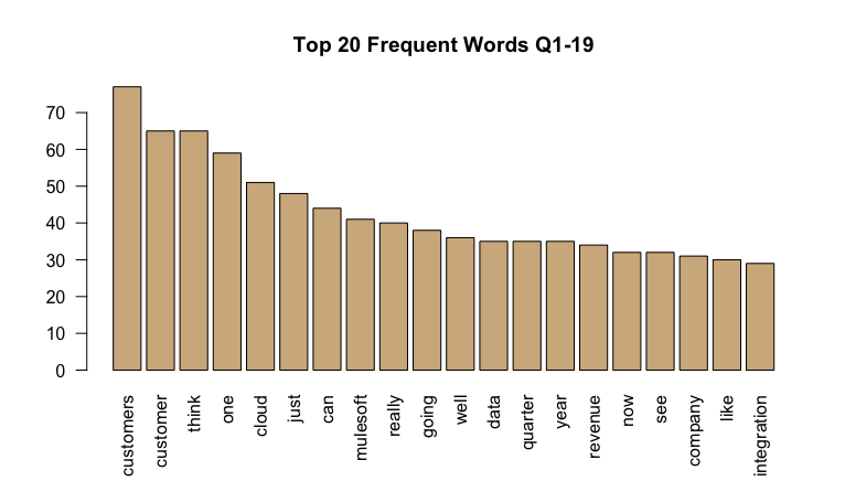
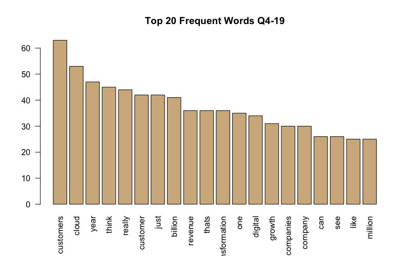
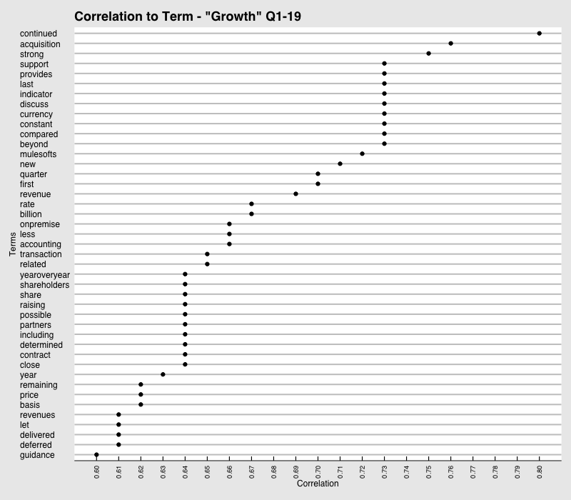
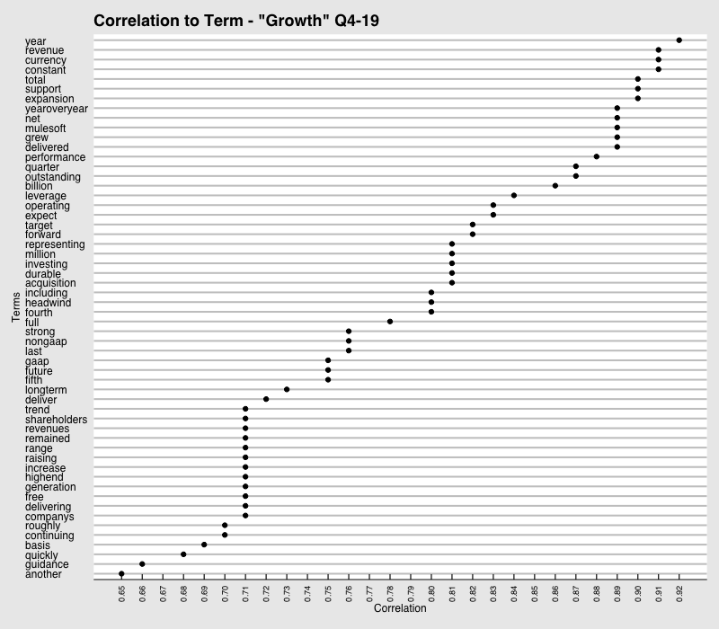
It looks like there is a common narrative associated with business operations such as “customers” cloud" and “one”. I will drop these words out of the text as they don’t uncover much. On the bright side, it’s a good thing to see that “growth” ranked #14 in the top 20 list for Q4-19. I want to possibly find any associations with specific keywords. Being that “growth” was ranked #14 in our list, I will choose this word to find associations/correlations with. The “tm” package also offers a function called ‘findAssocs’ that returns a vector that holds matching terms from x and their rounded correlations satisfying the inclusive lower correlation limit of corlimit. See below for the word associations using this function for the word “growth” in both Q1-19 and Q4-19 earnings transcripts.
#Running Sentiment Analysis From this point on, I will convert the data frame into a tibble, which is a different form of data frame that is easier to work with. After the tibble object is created, each set of text can be labeled according to if its text from an executive or an analyst.
#Create tibble object
tibble_tidy <- data.frame(doc_id = c(conf_call_df$names,qna_full$names), text = c(conf_call_df$text, qna_full$text)) %>% DataframeSource() %>% VCorpus() %>% tidy()


#Label according to who is speaking
z <- 0
for(i in tibble_tidy$id){
  z <- z+1
  if(i %in% analyst){
    tibble_tidy$author[z] <- "analyst"
  } else tibble_tidy$author[z] <- "management"
}


#Keep only the rows you are interested in
tibble_tidy <- tibble_tidy[,c("author", "id", "text")]

#Unnest tokens, which converts all text to lowercase, and seperates our text by word
text_tidy <- tibble_tidy %>% mutate(line_number = 1:nrow(.)) %>% group_by(author) %>% unnest_tokens(word, text) %>% ungroup()
Bing Lexicon: Scoring Sentiment from -1 to 1
Let’s view the different levels of sentiment starting with the simple “Bing” lexicon designed by Bing Liu, a distinguished professor at the University of Illinois at Chicago. This lexicon classifies words either negative or positive from a dictionary of 6,788 keywords. Let’s take a look at the 10 most frequent bing scored words in the Q1 transcript. First, I want to quickly glance at the words and type of sentiment. Then, I can look at the top 10 most common filtered words that are scored in the text.
#Bing lexicon
bing <- tidytext::get_sentiments("bing")

#We want to keep "great" as this is very positive in financial sentiment
stop_words <- tidytext::stop_words %>% filter(word != "great")

#Create tiddy object that is filtered and scored
text_tidy_bing <- text_tidy %>% inner_join(bing, by = "word") %>% anti_join(tidytext::stop_words, by = "word")

#Top 10 most frequent bing scored words in our text.
head(text_tidy_bing %>% count(word, sentiment, sort = TRUE),10)
## # A tibble: 10 x 3
## word sentiment n
## <chr> <chr> <int>
## 1 cloud negative 53
## 2 trust positive 22
## 3 guidance positive 14
## 4 incredible positive 13
## 5 success positive 12
## 6 innovation positive 11
## 7 intelligence positive 10
## 8 amazing positive 9
## 9 strong positive 8
## 10 top positive 8No surprise to see cloud mentioned 50 times being that salesforce business segments operate in the cloud. What’s MOST surprising is that the Bing dictionary considers this a negative word. Imagine if this slipped by, and “cloud” was labeled a negative contribution to the sentiment!
Adjusting the Database
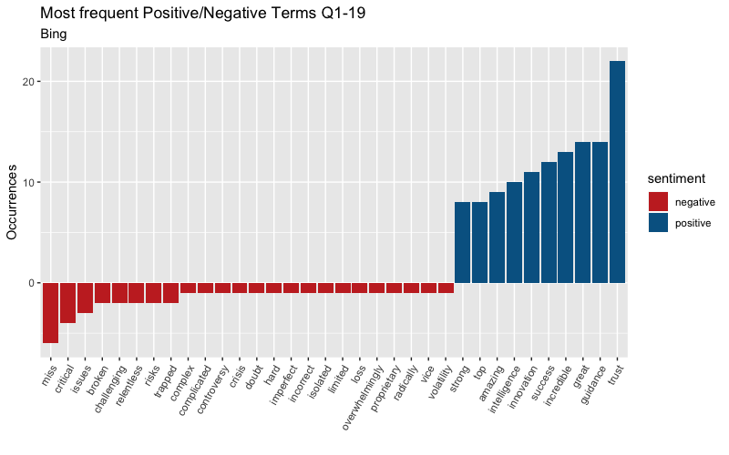
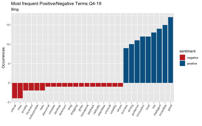
This can distort the sentiment outlook so I must be careful and look at words that are impacting the score the most. It is worth noting that this dictionary and others, will not always best fit our style of text as we can see. You should always analyze if whether or not it is in the dictionary your most frequent terms are in the dictionary and decide if it needs to be adjusted fit the industry and company that is under analysis. After quickly glancing through the top 50 frequent terms in the transcript, I noticed the term “headwinds” used in various quarters. In finance, headwinds are viewed as a negative term and will need to be adjusted the bing dictionary to score this negative term. We get can a cleaner view of positive vs negative terms once this is done. See below for a plot of the most frequent pos / neg terms used in Q1 & Q4.
Analysts vs Management: Bing
Were the analysts more positive than the management? Generally, management is mostly positive and attempts to shed light on any issues they may have. On the other hand, analysts are not as optimistic since it is their job to dig underneath the surface. I want to take a look at the overall positive/negative sentiment from Analysts and Management. Below is the code for Q1-19 plot but the picture is of Q1-19 & Q4-19.
#Seperate sentiment by author
author_sentiment_bing <- text_tidy_bing %>% count(author, sentiment) %>% group_by(author) %>%  mutate(percent = n / sum(n))


bingplot_q1 <- ggplot(author_sentiment_bing, aes(author, percent, fill = sentiment)) + geom_col() + theme(axis.text.x = element_text(angle = 0)) + labs(x = "Author", y = "Total Percentage",title = "Makeup of Positive/Negative Sentiment", subtitle="Bing: Q1-19")

gridExtra::grid.arrange(bingplot_q1,bingplot_q4,nrow=1)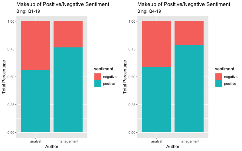
Sentiment Throughout Earnings Call
Now, I would love to see the sentiment throughout the conference call to see if there are any noticeable dips at any point. This could signal bad news or something that should be looked into further.
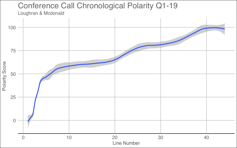
Sentiment or polarity is calculated by taking the positive-negative terms and dividing by the total # of positive/negative terms. Earning calls usually start off great due to management boasting any recent achievements, but once analysts begin to ask about future guidance or for more detail, you can see an initial slowdown in sentiment. We can see this below through the different plots of polarity over the course of the call.
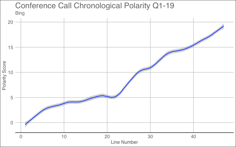
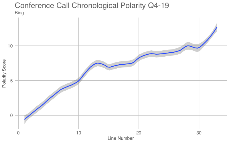
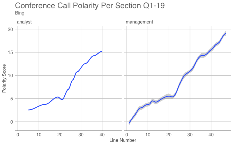
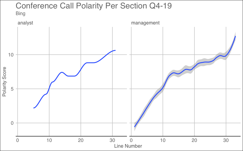
The above graphs are evidence for a conference call that had a positive sentiment. Later, I will check to see if this is true or not. In some cases, you will see a large dip in the score which could signal a very negative announcement that resulted in bad sentiment.
Afinn Lexicon: Scoring Sentiment from -5 to 5
Another lexicon used for sentiment analysis is the Afinn database. Its score has a scale of -5 to 5 based off sentiment for each of the 2,476 keywords. Some keywords hold larger weights with a score of five, while some hold a lighter weight of one. This lexicon was developed by a Danish researcher, Finn Arup Nielsen.
#Afinn lexicon
afinn <- tidytext::get_sentiments("afinn")

#Create tibble for AFINN
text_tidy_finn <- text_tidy %>% inner_join(afinn, by = "word") %>% anti_join(stop_words, by = "word") %>% mutate(sentiment=ifelse(score < 0, "negative","positive"))

#Of course we need to check for possible adjustments
head(text_tidy_finn %>% count(word,score, sort = T),100)
## # A tibble: 100 x 3
## word score n
## <chr> <int> <int>
## 1 growth 2 22
## 2 trust 1 22
## 3 ability 2 20
## 4 great 3 14
## 5 success 2 12
## 6 innovation 1 11
## 7 amazing 4 9
## 8 strong 2 8
## 9 top 2 8
## 10 vision 1 8
## # … with 90 more rowsThere is my favorite keyword, Growth!
Let’s now view the polarity throughout the conference call.
#Calculate total words per section (or line number)
total_words_finn <- text_tidy_finn %>% anti_join(stop_words, by = "word") %>% count(line_number,word) %>% group_by(line_number) %>% summarise(total_finn_words=sum(n))


#Calculate polarity over time of the call
afinn_scores <- text_tidy_finn %>% count(line_number,word,score) %>% group_by(line_number) %>% summarise(score = sum(score * n)) %>% inner_join(total_words_finn,by = "line_number") %>% mutate(polarity=cumsum(score/total_finn_words))


#Plot the overall polarity over the entire lentgth call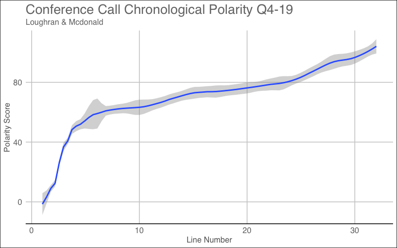
ggplot(afinn_scores, aes(line_number, polarity)) + geom_smooth(span = 0.2) + labs(x = "Line Number", y = "Polarity Score",title = "Conference Call Chronological Polarity Q4-19",subtitle="AFINN") + theme_gdocs() 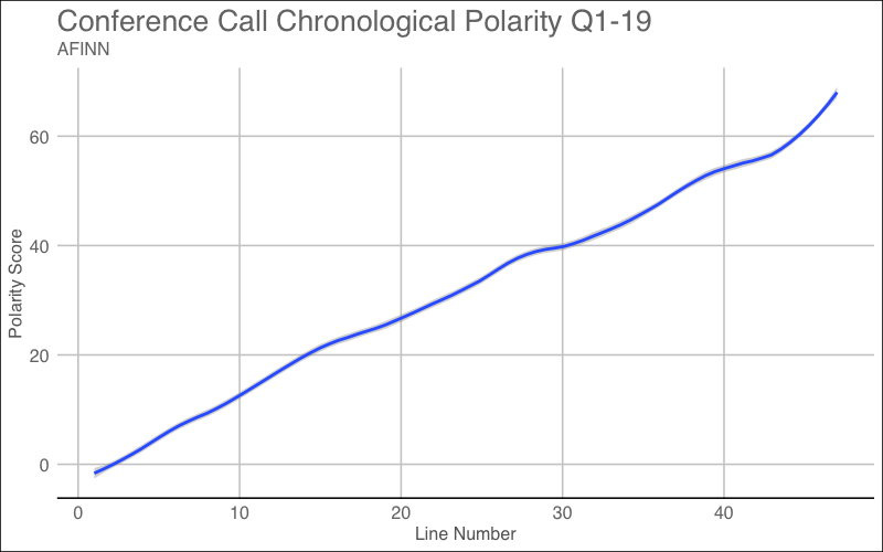
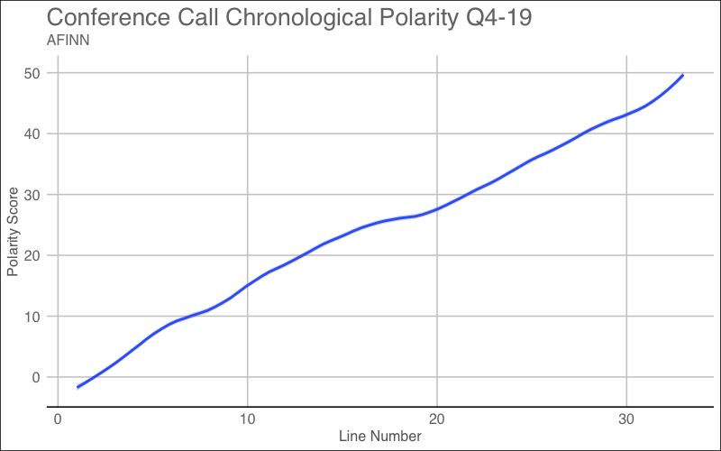
When the score is plotted over the entire length of the conference call, the trend shows the same characteristics as the Bing visualization. Just like in the Bing Sentiment chart, the overall sentiment score begins to increase from the start and continues into the end of the earnings call.
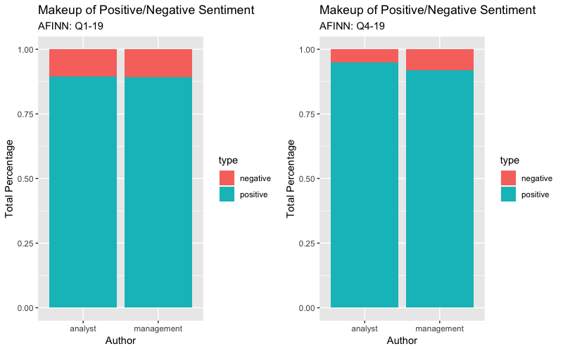
Analysts vs Management: Afinn
I want to take a look at the overall positive/negative sentiment from Analysts and Management. Below is the code for Q1-19 plot but the picture is of Q1-19 & Q4-19.
#Seperate sentiment by author
author_sentiment_finn <- text_tidy_finn %>% count(author, score) %>% mutate(tot_score=score*n) %>% mutate(type = ifelse(score < 0,"negative", "positive")) %>% group_by(author, type) %>% summarise(tot_word=sum(n)) %>% mutate(percent = tot_word / sum(tot_word))


#Plot each plot side by side
afinnplot_q1 <- ggplot(author_sentiment_finn, aes(author, percent, fill = type)) + geom_col() + theme(axis.text.x = element_text(angle = 0)) + labs(x = "Author", y = "Total Percentage",title = "Makeup of Positive/Negative Sentiment", subtitle="AFINN: Q1-19")


gridExtra::grid.arrange(afinnplot_q1, afinnplot_q4, nrow = 1)
Afinn Frequency Stacked Barplot
This also gives a similar view as the Bing database, but only because we plotted the frequency percentage of pos/neg key terms. I did not take into account the scores for each key term, so when comparing the new sentiment score vs the frequency of each positive/negative term we can see it shows a slightly different story.
#Seperate by author sentiments
author_sentiment_finn_scored <- text_tidy_finn %>% count(author, score) %>% mutate(tot_score=score*n) %>% mutate(type = ifelse(score < 0,"negative", "positive")) %>% group_by(author, type) %>% summarise(tot_score=sum(tot_score)) %>% mutate(tot_score=ifelse(tot_score<0,tot_score*-1,tot_score*1)) %>% ungroup() %>% group_by(author) %>% mutate(percent = tot_score / sum(tot_score))


#Plot each plot side by side
afinnplot_scored_q1 <- ggplot(author_sentiment_finn_scored, aes(author, percent, fill = type)) + geom_col() + theme(axis.text.x = element_text(angle = 0)) + labs(x = "Author", y = "Total Percentage",title = "Makeup of Positive/Negative Sentiment", subtitle="AFINN: Q1-19")


gridExtra::grid.arrange(afinnplot_scored_q1, afinnplot_scored_q4, nrow = 1)
Afinn Scored Stacked Barplot
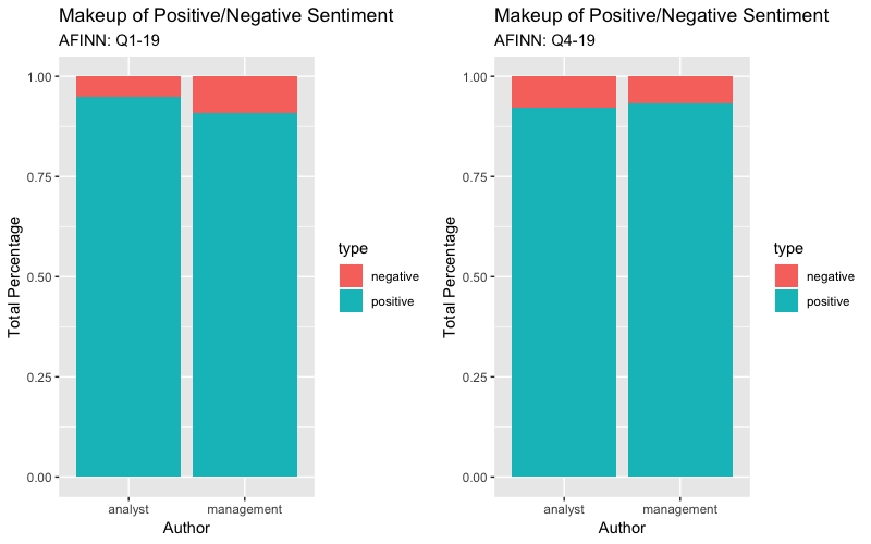
Using the new total sentiment score, it shows a slightly different narrative than the frequency graph above. In Q1, the analysts were slightly more positive than the management while the scored graph showed a wider difference. In Q4, the analysts were a little more positive than the management but the scored graph shows management having more positive tone in sentiment. This shows that the -5 to 5 scoring scale is effective in scoring some words with a higher weight than others.
NRC Lexicon: Sentiment Emotions
Another form of sentiment analysis can classify the emotion of the speaker by using NRC lexicon. This lexicon scores a distinct emotional class covering Plutchiks Wheel of Emotions. The NRC lexicon, developed by Saif Mohammad and Peter Turney, consists of 13,901 keywords and also includes positive and negative words. Since I’ve already done positive and negative scoring scales words, we will subset this type of scoring out and only analyze the remaining 8,265 key emotion words. Of course, I need to look at the biggest contributors to the score and if it is appropriate for our text.
#NRC lexicon
nrc <- tidytext::get_sentiments("nrc")

nrc_score_tidy <- text_tidy %>% inner_join(nrc, by = "word") %>% anti_join(stop_words, by = "word")

#Check for possible adjustments
head(nrc_score_tidy %>% count(word,sentiment, sort = T),100)
## # A tibble: 100 x 3
## word sentiment n
## <chr> <chr> <int>
## 1 customer positive 65
## 2 growth positive 22
## 3 system trust 22
## 4 trust trust 22
## 5 commerce trust 21
## 6 ability positive 20
## 7 continue anticipation 14
## 8 continue positive 14
## 9 continue trust 14
## 10 guidance positive 14
## # … with 90 more rowsWe can see the sentiment score scale change from integer to a categorical value. Since the executives have more airtime on these calls, they will have more words to count from so we will log the values to normalize the scale. I want to use a radar chart to view the overall emotions of the executives and analysts. Below is the code for creating the Q1 grouped NRC df, but the plots show both Q1 & Q4. I will also show stacked bar charts for comparison.
nrc_scores_group_radar_q1 <- nrc_score_tidy %>% filter(!grepl("positive|negative", sentiment)) %>% count(author, sentiment) %>% spread(author,n)#Plot radar chart to view NRC scores
radarchart::chartJSRadar(nrc_scores_group_radar_q1, main = "Wheel of Emotions Q1-19")#Plot radar chart to view NRC scores
radarchart::chartJSRadar(nrc_scores_group_radar_q4, main = "Wheel of Emotions Q4-19")
It looks like NONE of the analysts sounded sad in Q1 or Q4! The management had the highest tone of Joy throughout the conference call. Overall, I would say that anticipation and trust seemed to be the overall emotion for the length of the call. I am not a big fan of this lexicon, as the emotions of the analysts or management at the time of call doesn’t tell much regarding the long term future of the company.
The Famous Loughran & Mcdonald Lexicon
This lexicon contains 2702 key terms that relate to business operations. This lexicon is a list of positive, negative and uncertainty words according to the Loughran-McDonald finance-specific dictionary. This dictionary was first presented in the Journal of Finance and has been widely used in the finance domain ever since. In the “lexicon” package, we can load this lexicon which classifies “uncertainty” words as negative values. We could also use the “SentimentAnalysis” package that supplies only the words of the lexicon. First, I want to view the Top 10 most frequent scored keywords.
#Loughran & Mcdonald lexicon
loughran_mcdonald <- lexicon::hash_sentiment_loughran_mcdonald


#Create tiddy object that is filtered and scored
text_tidy_hash_sentiment_loughran_mcdonald <- text_tidy %>% inner_join(loughran_mcdonald, by = c("word" = "x")) %>% anti_join(stop_words, by = "word")


#Top 10 most frequent loughran_mcdonald scored words in our text.
head(text_tidy_hash_sentiment_loughran_mcdonald %>% count(word, y, sort = TRUE),10)
## # A tibble: 10 x 3
## word y n
## <chr> <dbl> <int>
## 1 great 1 14
## 2 incredible 1 13
## 3 question -1 12
## 4 success 1 12
## 5 innovation 1 11
## 6 strong 1 8
## 7 tremendous 1 8
## 8 leading 1 7
## 9 miss -1 6
## 10 achieve 1 4Great! These type of keywords are more business oriented which is a great fit for conference call analysis. One thing that is not a great fit is the negative score placed on the word “question” which I will need to adjust.
After adjusting, I want to illustrate the top positive/negative scored terms.
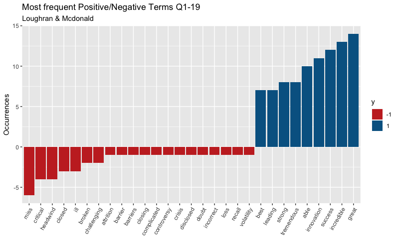
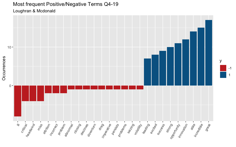
It looks like this dictionary scores the word “ill” as a negative term which makes sense. During my text cleanup, I changed all of “I’ll” to “ill” which is being scored as a negative. You must always pay attention to detail even after you’ve cleaned your text! I will adjust for this as well and illustrate the polarity score throughout the conference call below.
Overall Lexicon Sentiment Results
We can see from the final lexicon, that the sentiment throughout the call also shared similar characteristics to the other lexicons. Now that I have visualized all four sentiments from each lexicon, I want to take a look at a data frame with the earnings dates, positive scored words, negative scored words, total words, overall scores, positive/negative sentiment, lexicon, and even the adjusted 3-month forward adjusted returns. This is something I was saving behind the scenes as I analyzed each lexicon.
print.data.frame(sentiment_df)## Ticker Earnings_date Positive Negative Total_words
## 1 CRM May 29, 2018 8:53 PM ET 276 92 10142
## 2 CRM May 29, 2018 8:53 PM ET 309 37 10142
## 3 CRM May 29, 2018 8:53 PM ET 580 59 10142
## 4 CRM May 29, 2018 8:53 PM ET 146 47 10142
## 5 CRM Aug. 29, 2018 9:54 PM ET 280 88 8646
## 6 CRM Aug. 29, 2018 9:54 PM ET 277 30 8646
## 7 CRM Aug. 29, 2018 9:54 PM ET 509 57 8646
## 8 CRM Aug. 29, 2018 9:54 PM ET 139 47 8646
## 9 CRM Nov. 28, 2018 12:01 AM ET 314 102 9496
## 10 CRM Nov. 28, 2018 12:01 AM ET 309 37 9496
## 11 CRM Nov. 28, 2018 12:01 AM ET 539 93 9496
## 12 CRM Nov. 28, 2018 12:01 AM ET 157 46 9496
## 13 CRM Mar. 4, 2019 11:53 PM ET 282 85 8953
## 14 CRM Mar. 4, 2019 11:53 PM ET 312 26 8953
## 15 CRM Mar. 4, 2019 11:53 PM ET 538 59 8953
## 16 CRM Mar. 4, 2019 11:53 PM ET 152 40 8953
## Score Sentiment Lexicon fwd_qtr_return
## 1 19.0045208 positive bing 0.1832173
## 2 67.6090723 positive afinn 0.1832173
## 3 0.8153365 positive nrc 0.1832173
## 4 0.5129534 positive loughran_mcdonald 0.1832173
## 5 14.8544156 negative bing -0.1691205
## 6 44.8652201 negative afinn -0.1691205
## 7 0.7985866 negative nrc -0.1691205
## 8 0.4946237 negative loughran_mcdonald -0.1691205
## 9 18.6783881 positive bing 0.1269909
## 10 67.6090723 positive afinn 0.1269909
## 11 0.7056962 negative nrc 0.1269909
## 12 0.5467980 positive loughran_mcdonald 0.1269909
## 13 12.6184193 negative bing NA
## 14 49.7076174 negative afinn NA
## 15 0.8023451 positive nrc NA
## 16 0.5833333 positive loughran_mcdonald NALooking at whether the score classified the transcript as positive or negative, I can see how accurate the classification was by comparing that to the adjusted 3-month forward return. If the transcript was classified as positive, then loosely speaking, that should translate to positive stock performance going into the following quarter. We can see that the NRC emotion lexicon failed to correctly classify one out of three transcripts while the other lexicons classified all three correctly according to adjusted forward returns. The four NA’s are for the current quarter since the full 3-month adjusted return does not exist yet.
Tokenization
Tokenization helps to divide the text into individual words. For performing tokenization process, there are many open source tools are available. Tokenization is the process of breaking a stream of textual content up into words, terms, symbols, or some other meaningful elements called tokens. During this post, I’ve only analyzed single-words that breaks up the text into one-word “tokens”. Now, I want to look at a variety of bi-gram and tri-gram tokens, or two-word / three-word phrases.
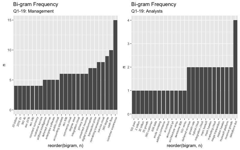
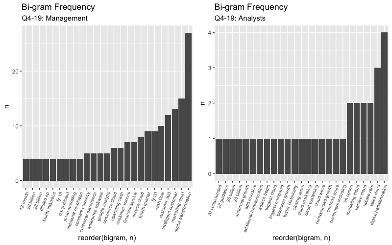
Bi-gram
I can increase the amount of “tokens” or words that we use when building our n-grams which would result in bi-gram, or a tri-gram for three-word phrases. Also, I can check for any negation words that may arrive before any of the highest positive words to see if anything needs to be adjusted. This is a bit more sophisticated than a single word analysis. If growth occurs 20x in a text, can I say that it is positive? Not exactly, because what if “slow growth” occurred 15 out of those 20 times. At the end of creating the bi-gram, I can check for any negation words that occur before any of our scored keywords.
Most frequent bi-grams with “growth”
#Create Bi-gram tibble. This creates a row for every bi-gram, or two-word phrase.
text_tidy_bi <- tibble_tidy %>% mutate(line_number = 1:nrow(.)) %>% group_by(author) %>% unnest_tokens(bigram, text, token = "ngrams", n = 2) %>% ungroup() %>% arrange(line_number)


#Seperate the bi-gram column into two column, one for each word. Filter for stop words.
text_tidy_bi_filtsep <- text_tidy_bi %>% separate(bigram, c("word1", "word2"), sep = " ") %>% filter(!word1 %in% stop_words$word & !word2 %in% stop_words$word)


#Count most common bi-gram associated with groth
text_tidy_bi_filtsep %>% filter(word2 == "growth" | word2 == "growing" | word1 == "growing" | word1 == "growth" | word2 == "grow" | word1 == "grow") %>% count(word1, word2, sort = TRUE)
## # A tibble: 23 x 3
## word1 word2 n
## <chr> <chr> <int>
## 1 growth rate 6
## 2 revenue growth 3
## 3 fastest growing 2
## 4 remarkable growth 2
## 5 25 growth 1
## 6 35 growth 1
## 7 amazing growth 1
## 8 apples growth 1
## 9 basis growing 1
## 10 cloud growth 1
## # … with 13 more rowsChecking for negation words
How often are words preceded by a word like “not” or “no” and is the score conflicting? I found none in the Q1 call but see below for what I found in Q4.
#Seperate the bi-gram column into two columns but do not adjust for stop words to properly search for negation words.
text_tidy_bi_sep <- text_tidy_bi_q4 %>% separate(bigram, c("word1", "word2"), sep = " ")

#Afinn
afinn <- tidytext::get_sentiments("afinn")

#negation words before scored key word
text_tidy_bi_sep %>% filter(word1 %in% qdapDictionaries::negation.words) %>% inner_join(afinn, by = c(word2 = "word"))
## # A tibble: 1 x 6
## author id line_number word1 word2 score
## <chr> <chr> <int> <chr> <chr> <int>
## 1 management Mark Hawkins 10 not perfectly 3Only one negation word in Q4 occured before any of our scored key words which was “not”. The key word was perfectly and this bi-gram occured 3 times. I do not think this needs to be accounted for but we can double check when analyzing “tri-grams”.
Tri-gram
Moving from Bi-gram to Tri-gram, we can expect the same concept as bi-grams but with a little more power. We can now check for 3-word phrases and analyze before and after a scored keyword.
#Create Tri-gram tibble. This creates a row for every tri-gram, or three-word phrase.
text_tidy_tri <- tibble_tidy %>% mutate(line_number = 1:nrow(.)) %>% group_by(author) %>% unnest_tokens(trigram, text, token = "ngrams", n = 3) %>% ungroup() %>% arrange(line_number)

#Seperate the bi-gram column into two column, one for each word. Filter for stop words.
tri_words <- text_tidy_tri %>% separate(trigram, c("word1", "word2", "word3"), sep = " ") %>% filter(!word1 %in% stop_words$word & !word2 %in% stop_words$word & !word3 %in% stop_words$word) %>% unite(trigram, word1, word2, word3, sep = " ")

#Count 10 most common tri-gram phrases.
tri_words %>% count(trigram, sort = TRUE) %>% head(10)
## # A tibble: 10 x 2
## trigram n
## <chr> <int>
## 1 remaining transaction price 7
## 2 360 degree view 6
## 3 asc 2016 01 4
## 4 asc 340 40 4
## 5 field service lightning 4
## 6 national privacy law 4
## 7 operating cash flow 4
## 8 2 billion predictions 3
## 9 accounting standards asc 3
## 10 current remaining transaction 3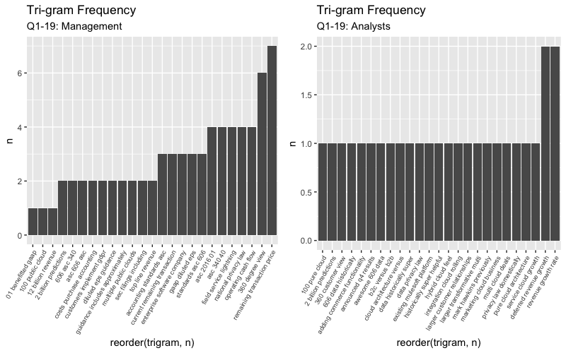
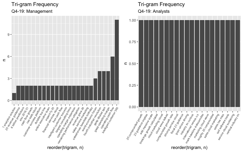
These charts look similar to each other from Q1 to Q4, but after taking a closer look you can see the tri-gram phrases differ. It seems like the management switched focus from covering the mulesoft acquisition “remaining transction price” in Q1 to now focusing on creating an all-in-one or “customer 360” platform in the most recent Q4 call.
Checking for negation words
How often are words preceded by a word like “not” or “no” and is the score conflicting? I found none in the Q1 call but see below for what I found in Q4.
#Afinn lexicon as scored words
afinn <- tidytext::get_sentiments("afinn")


#Check negation words in word1 or word2 while joining to scored keywords by word 3
text_tidy_tri_q4 %>% separate(trigram, c("word1", "word2", "word3"), sep = " ") %>% filter(word1 %in% qdapDictionaries::negation.words | word2 %in% qdapDictionaries::negation.words) %>% inner_join(afinn, by = c(word3 = "word"))
## # A tibble: 1 x 7
## author id line_number word1 word2 word3 score
## <chr> <chr> <int> <chr> <chr> <chr> <int>
## 1 management Mark Hawkins 10 is not perfectly 3#Check negation words in word1 while joining to scored keywords by word 2
text_tidy_tri_q4 %>% separate(trigram, c("word1", "word2", "word3"), sep = " ") %>% filter(word1 %in% qdapDictionaries::negation.words) %>% inner_join(afinn, by = c(word2 = "word"))## # A tibble: 1 x 7
## author id line_number word1 word2 word3 score
## <chr> <chr> <int> <chr> <chr> <chr> <int>
## 1 management Mark Hawkins 10 not perfectly comparable 3Remember the “not perfectly” Negator bi-gram that we saw? By using a tri-gram, I can shed more light on the bi-gram that saw a negation word before the keyword. As we can see with a score of only 3, the complete phrase of “not perfectly comparable” is something that doesn’t need much attention, compared to something like “not growing revenue” which may signal red flags.
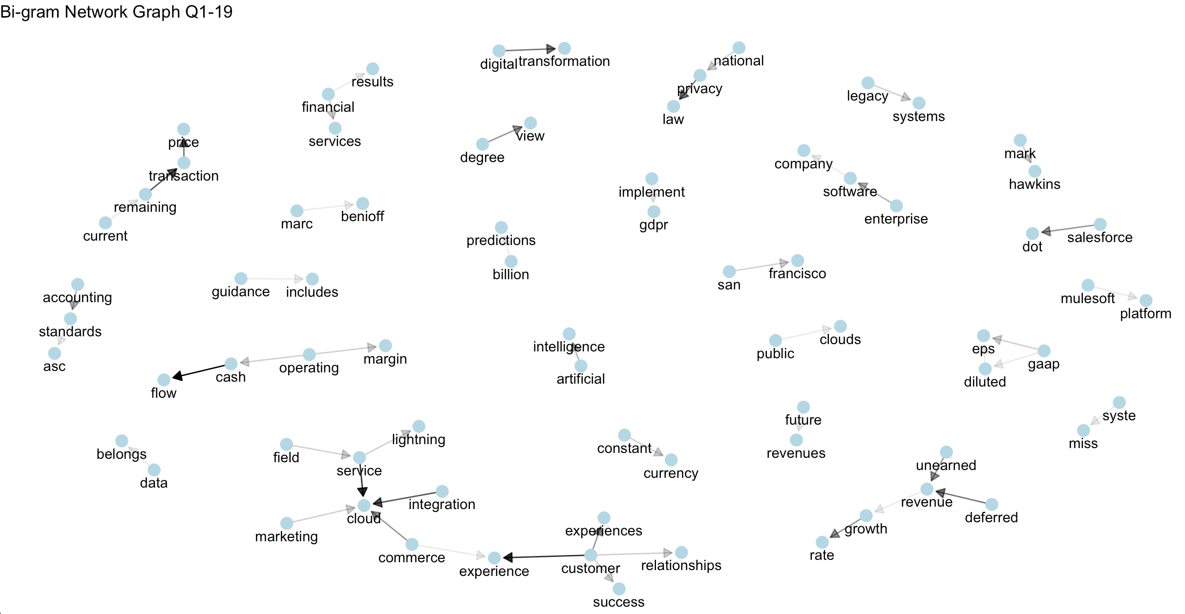
Visualizing Textual Relationships
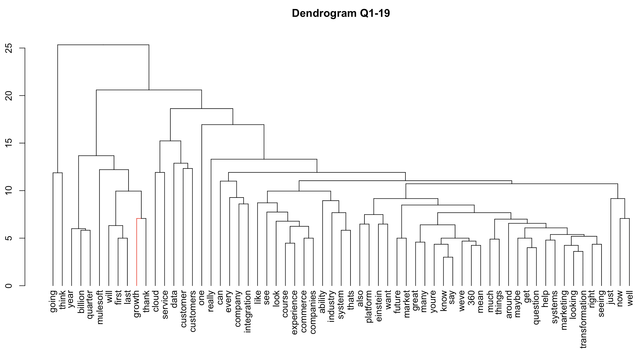
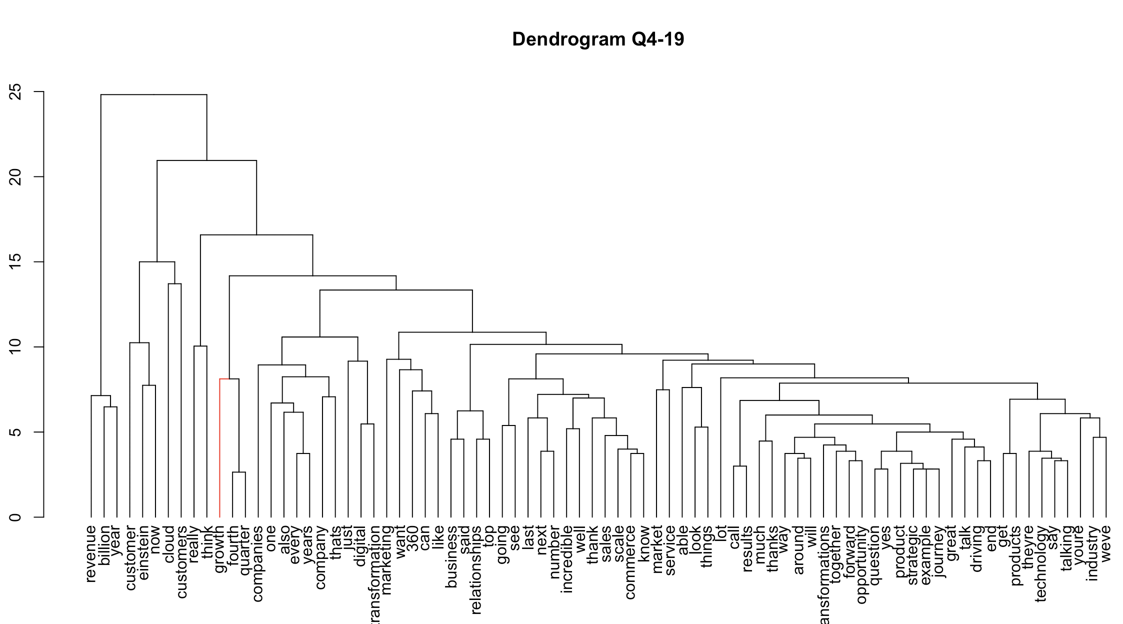
Viewing relationships in the text through Network Graphs, Dendrograms, and Correlation Networks can be helpful to find unusual relationships. You can edit these to fit the patterns you are looking for, which I will continue to search for “growth” keywords. Without going into too much detail regarding these graphs, they are all attempting to show the relationships between the text. If the words share a strong relationship, you will see them clustered together or near each other on the below charts.
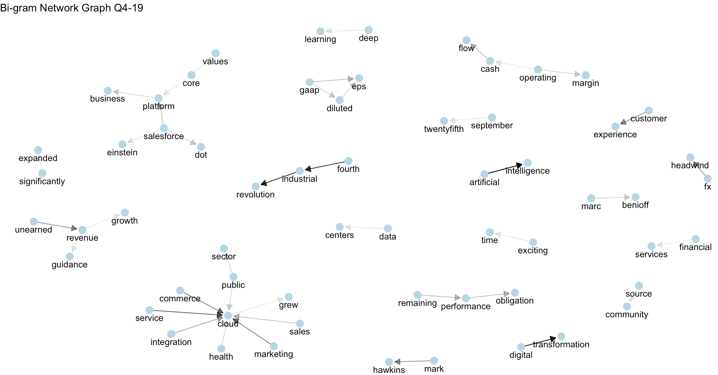
Network graphs
Dendrograms
Correlation with the word “Growth” Q1-19
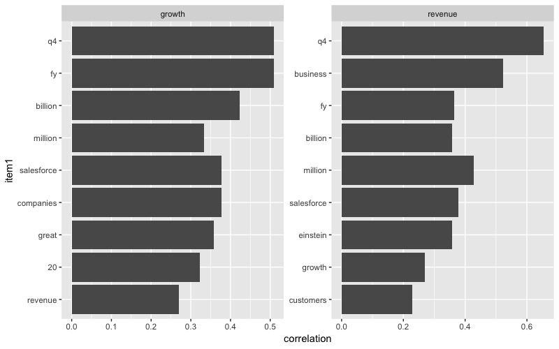
Correlation with the word “Growth” Q4-19
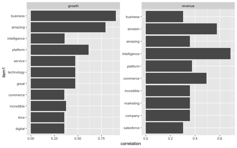
Remember how we saw the word “headwind” appear in our text but not in the scoring lexicons? Well, these visualizations exploit the cause of these “headwinds” which was FX as seen in the Q4 network graph. I can also see relationships such as “grew revenue”, “durable growth” and “incredible innovation”. These can be extremely powerful, especially in situations where I have a set of words that I want to find any relationships for or correlations within the text. I would highly suggest those who are interested in these charts to read more details on how these relationships are found.
Looking Forward
After reading “Forecasting Returns Using Earnings Call Transcripts”, I was inspired to consider a similar approach. I wanted to create multiple lists of words/phrases as a lexicon that represent factors which could drive excess returns to the set of stocks I am following. Since Salesforce is considered a growth stock, I would consider looking for growth factors and operational factors such as revenue growth, margin expansions, improved operating leverage, etc. We can count the number of terms that occurred within each of these categories, total terms within the document, and begin calculating scores for each of those categories in each transcript. The idea is to use a regression using the scores against the forward adjusted returns to find the optimal weights to use for each category.
Once I can get a sentiment analysis model similar to the Stanford research project, my plan is to run a few different analysis to test which lexicon approach is best to use for conference call sentiment analysis. This type of work and detail will need to be saved for the part 2 post, so stay tuned!!
