
Using Airbnb
By now, most Gen Z and millenials have heard of or used Airbnb for a range of many reasons, such as looking for a place to crash or taking a vacation. I believe what won the consumer’s attention over hotels was the fact that you are getting the “homey” setting and privacy while away on vacation instead of a hotel environment. I realize not everyone wants to part ways with room service, benefits of a having full-service bar in the lobby, pool & spas, sometimes a gym, and the 100+ channels, but when comparing the prices and the extra sq. footage, it is hard not to take a look at and possibly book Airbnb listings.
Listing on Airbnb
While most of us have used or considered booking an Airbnb, there are a lot less of us who have considered posting our own property on Airbnb. Being that New York City rent is extremely high, I’ve considered listing my Brooklyn apartment to see what kind of profits I could turn. During this time, I was learning about multiple linear regression in my Quantitative Analysis & Forecasting class and was assigned a project to create a linear model to predict some form of dependent variable. I figured why not use this opportunity to dig a little deeper on estimating a listing price for my apartment. This led me to stumble upon pretty interesting information about commercial operators listings on Airbnb in New York City. To keep this post in line with the subject, I will just quickly summarize what I found in the following paragraph.
Commercial Operators
What exactly is a commercial operator? This is an Airbnb host that has multiple entire-home listings or controls many private-room listings. If I was to post on Airbnb to try and squeeze a profit, I would list my property for certain days or weeks of the month, and at most a rental property if I happened to own one. This compares to commercial operators who may have 4-6 entire home listings and 8-12 private room listings. It was estimated that commercial operators make up 12% of NYC Airbnb hosts, but earned almost 1/3 of all incoming revenue.
Why is this an issue?
I believe it is an issue because it is depleting the actual prices hosts could get for their properties if they were to list on Airbnb. If it weren’t for commercial operators saturating the market with these lower-priced listings, maybe I could squeeze an extra $20-30/ night from my listing. Think of these NYC commercial operators as the Walmart or Amazon of property listings. They often charge less per night than other hosts do across all listings and adjust their rates to attract a high number of rentals overall. To summarize, they are flooding the New York City markets with lower-priced listings.
Now the fun stuff - Building the Model
I found my data off of InsideAirBnb.com which is an independent, non-commercial set of tools and data that allows you to explore how Airbnb is really being used in cities around the world. I retrieved all listings in NYC as of 03/2018. This was a very large data set that contained 29,142 listings in NYC with 96 different factors to choose from as my independent variables. I would like to keep in mind the effect commercial operators have on prices. I believe that Airbnb listing prices are not fully predictable by the usual variables one would use to predict the price of a traditional property in NYC. These usual variables are factors such as bedroom count, bathroom, location, property type, and etc. If the listing prices were fully explainable by these usual variables, then I would assume with our data we will be able to train and build our model strong enough to have a low root mean squared error (RMSE). See below for how I got to our final Model.
The Process
After loading in the data, I began to analyze the structure to search for any outliers or missing values. Our initial data set has a dimension of 29142 rows and 96 columns so let’s begin cutting down the amount of factors playing into the pricing. I will choose the variables that make the most sense when predicting a price for a property.
Cleaning the Data
trimData <-subset(data,select = c("price"
                                  ,"cancellation_policy"
                                  ,"is_business_travel_ready"
                                  ,"accommodates"
                                  ,"bedrooms"
                                  ,"beds"
                                  ,"bathrooms"
                                  ,"number_of_reviews"
                                  ,"instant_bookable"
                                  ,"review_scores_rating"
                                  ,"review_scores_location"
                                  ,"review_scores_cleanliness"
                                  ,"review_scores_checkin"
                                  ,"review_scores_value"
                                  ,"neighbourhood_group_cleansed"
                                  ,"neighbourhood_cleansed"
                                  ,"room_type"
                                  ,"availability_30"
                                  ,"availability_365"
                                  ,"calculated_host_listings_count"
                                  ,"reviews_per_month"
                                  ,"host_is_superhost"
                                  ,"host_identity_verified"
                                  ,"host_listings_count"
                                  ,"cleaning_fee"
                                  ,"guests_included"
                                  ,"zipcode"
                                  ,"property_type"))
Take out all observations with Price equal to $0 and 0 days availbility within the next year. Also, check and remove any observations with NA’s as values
non0data <- subset(trimData, price != 0 & availability_365 != 0)
sapply(non0data, function(x) sum(is.na(x)))
## price cancellation_policy
## 0 0
## is_business_travel_ready accommodates
## 0 0
## bedrooms beds
## 0 9
## bathrooms number_of_reviews
## 0 0
## instant_bookable review_scores_rating
## 0 0
## review_scores_location review_scores_cleanliness
## 0 0
## review_scores_checkin review_scores_value
## 0 0
## neighbourhood_group_cleansed neighbourhood_cleansed
## 0 0
## room_type availability_30
## 0 0
## availability_365 calculated_host_listings_count
## 0 0
## reviews_per_month host_is_superhost
## 0 0
## host_identity_verified host_listings_count
## 0 0
## cleaning_fee guests_included
## 2904 0
## zipcode property_type
## 0 0non0data <- non0data[complete.cases(non0data),]Let’s take a look at the big picture of our variables once more to double check that nothing is off
str(non0data)## 'data.frame': 17361 obs. of 28 variables:
## $ price : int 95 70 104 374 60 175 90 60 195 269 ...
## $ cancellation_policy : Factor w/ 5 levels "flexible","moderate",..: 2 1 2 3 3 3 3 1 3 2 ...
## $ is_business_travel_ready : Factor w/ 2 levels "f","t": 1 1 1 1 1 1 1 1 1 1 ...
## $ accommodates : int 2 2 2 5 3 2 4 2 1 2 ...
## $ bedrooms : int 1 1 1 2 1 0 1 1 0 1 ...
## $ beds : int 1 1 1 5 2 1 2 1 1 1 ...
## $ bathrooms : num 1 1 1 1 3 1 1 1 1 1 ...
## $ number_of_reviews : int 101 8 4 16 37 1 2 11 3 69 ...
## $ instant_bookable : Factor w/ 2 levels "f","t": 2 2 1 1 2 2 2 1 1 1 ...
## $ review_scores_rating : int 93 89 87 95 93 100 100 89 100 97 ...
## $ review_scores_location : int 8 9 10 10 9 10 10 9 10 10 ...
## $ review_scores_cleanliness : int 9 10 9 9 9 10 8 9 10 10 ...
## $ review_scores_checkin : int 10 9 10 10 10 10 10 10 10 10 ...
## $ review_scores_value : int 9 9 10 9 9 10 10 9 10 10 ...
## $ neighbourhood_group_cleansed : Factor w/ 5 levels "Bronx","Brooklyn",..: 3 3 3 3 1 3 2 1 3 3 ...
## $ neighbourhood_cleansed : Factor w/ 212 levels "Allerton","Arden Heights",..: 59 200 195 196 76 172 89 199 196 142 ...
## $ room_type : Factor w/ 3 levels "Entire home/apt",..: 2 2 1 1 2 1 1 2 1 1 ...
## $ availability_30 : int 3 12 4 27 22 3 10 29 0 6 ...
## $ availability_365 : int 74 182 244 362 357 22 10 364 9 313 ...
## $ calculated_host_listings_count: int 3 1 1 1 5 1 1 1 1 1 ...
## $ reviews_per_month : num 2.33 1 0.17 0.54 3.03 0.48 0.63 1.3 0.13 3.07 ...
## $ host_is_superhost : Factor w/ 2 levels "f","t": 2 1 1 1 1 1 1 1 1 2 ...
## $ host_identity_verified : Factor w/ 2 levels "f","t": 2 1 2 2 2 1 1 1 1 2 ...
## $ host_listings_count : int 3 1 1 1 5 1 1 1 1 1 ...
## $ cleaning_fee : int 50 20 60 200 20 100 35 25 70 120 ...
## $ guests_included : int 2 1 1 1 2 1 2 1 1 2 ...
## $ zipcode : Factor w/ 190 levels "","07002","07093",..: 31 35 44 25 81 17 120 80 25 16 ...
## $ property_type : Factor w/ 35 levels "Aparthotel","Apartment",..: 2 2 2 2 20 2 2 2 2 2 ...We can notice that under zip codes, there is a zip code titled "" with no value. Let’s take a closer look
length(non0data$zipcode[non0data$zipcode == ""])## [1] 202- We have 202 listings with no zip code. Since zip code can play a large role in the listing price, we will also take these listings out.
non0data$zipcode[non0data$zipcode == ""] <- NA
non0data <- non0data[complete.cases(non0data),]
Now that we have cleaned all of our data, we are ready to begin creating the model
- As expected, this model has a very high R^2 of .7709 most likely due to the fact that we have 26 independent variables. We notice that not all are statistically significant so we begin to remove those from the model.
model2 = lm(log(price)~log(accommodates)
           +bedrooms
           +beds
           +bathrooms
           +log(number_of_reviews)
           +review_scores_rating
           +review_scores_location
           +review_scores_cleanliness
           +log(review_scores_value)
           +neighbourhood_group_cleansed + room_type
           +availability_30
           +availability_365
           +calculated_host_listings_count
           +log(reviews_per_month)
           +host_is_superhost
           +host_identity_verified
           +cleaning_fee
           +guests_included
           +zipcode
           +property_type
,non0data)- Although model2 still has a very high R^2 of .7705, it still also has a lot of insignificant variables due to the fact that zip code consists of 190 levels and property_type has a bunch of insignificant property_types. I will substitute zip code for neighborhood_group_cleansed since it has 4 levels compared to 190 and I will remove all insignificant property_types.
uncommon_listings <- c("Tiny house", "Earth house", "Tent", "Timeshare", "Boat", "Chalet", "Hostel", "Train", "Cabin", "Treehouse", "Bungalow", "Castle", "Bed and breakfast", "Cave", "Casa particular (Cuba)", "Villa", "Boutique hotel", "Other", "In-law", "Camper/RV", "Yurt")

for (i in uncommon_listings){
  non0data <- subset(non0data, property_type != i)
}
Run Model 3 and veiw summary / coefficients
model3 = lm(log(price)~log(accommodates)
           +bedrooms
           +beds
           +bathrooms
           +log(number_of_reviews)
           +review_scores_rating
           +neighbourhood_group_cleansed + room_type
           +availability_30
           +availability_365
           +calculated_host_listings_count
           +host_is_superhost
           +host_identity_verified
           +cleaning_fee
           +guests_included
           +property_type
           ,non0data)
summary(model3)
##
## Call:
## lm(formula = log(price) ~ log(accommodates) + bedrooms + beds +
## bathrooms + log(number_of_reviews) + review_scores_rating +
## neighbourhood_group_cleansed + room_type + availability_30 +
## availability_365 + calculated_host_listings_count + host_is_superhost +
## host_identity_verified + cleaning_fee + guests_included +
## property_type, data = non0data)
##
## Residuals:
## Min 1Q Median 3Q Max
## -3.0552 -0.2266 -0.0001 0.2291 2.4700
##
## Coefficients:
## Estimate Std. Error t value
## (Intercept) 3.868e+00 1.882e-01 20.548
## log(accommodates) 2.185e-01 8.910e-03 24.525
## bedrooms 1.152e-01 5.528e-03 20.836
## beds -2.495e-02 4.134e-03 -6.037
## bathrooms 8.751e-02 7.065e-03 12.386
## log(number_of_reviews) -1.359e-02 2.233e-03 -6.086
## review_scores_rating 5.492e-03 4.037e-04 13.602
## neighbourhood_group_cleansedBrooklyn 2.498e-01 1.999e-02 12.497
## neighbourhood_group_cleansedManhattan 5.795e-01 2.025e-02 28.621
## neighbourhood_group_cleansedQueens 1.542e-01 2.108e-02 7.317
## neighbourhood_group_cleansedStaten Island -5.315e-02 3.820e-02 -1.391
## room_typePrivate room -5.025e-01 8.026e-03 -62.614
## room_typeShared room -9.280e-01 2.114e-02 -43.902
## availability_30 4.908e-03 2.933e-04 16.731
## availability_365 1.734e-04 2.542e-05 6.822
## calculated_host_listings_count -2.096e-02 1.526e-03 -13.737
## host_is_superhostt 4.006e-02 7.183e-03 5.577
## host_identity_verifiedt 4.739e-02 5.981e-03 7.923
## cleaning_fee 2.737e-03 8.073e-05 33.908
## guests_included 2.233e-02 2.719e-03 8.215
## property_typeApartment -4.753e-01 1.826e-01 -2.602
## property_typeCondominium -2.917e-01 1.843e-01 -1.582
## property_typeDorm -5.252e-01 2.237e-01 -2.348
## property_typeGuest suite -5.082e-01 1.873e-01 -2.713
## property_typeGuesthouse -6.010e-01 1.952e-01 -3.078
## property_typeHotel 4.794e-01 2.109e-01 2.273
## property_typeHouse -5.185e-01 1.828e-01 -2.836
## property_typeLoft -3.095e-01 1.834e-01 -1.688
## property_typeResort 5.806e-01 2.791e-01 2.080
## property_typeServiced apartment -3.504e-01 1.867e-01 -1.877
## property_typeTownhouse -5.195e-01 1.832e-01 -2.836
## property_typeVacation home -3.264e-01 2.358e-01 -1.384
## Pr(>|t|)
## (Intercept) < 2e-16 ***
## log(accommodates) < 2e-16 ***
## bedrooms < 2e-16 ***
## beds 1.60e-09 ***
## bathrooms < 2e-16 ***
## log(number_of_reviews) 1.18e-09 ***
## review_scores_rating < 2e-16 ***
## neighbourhood_group_cleansedBrooklyn < 2e-16 ***
## neighbourhood_group_cleansedManhattan < 2e-16 ***
## neighbourhood_group_cleansedQueens 2.65e-13 ***
## neighbourhood_group_cleansedStaten Island 0.16414
## room_typePrivate room < 2e-16 ***
## room_typeShared room < 2e-16 ***
## availability_30 < 2e-16 ***
## availability_365 9.31e-12 ***
## calculated_host_listings_count < 2e-16 ***
## host_is_superhostt 2.49e-08 ***
## host_identity_verifiedt 2.46e-15 ***
## cleaning_fee < 2e-16 ***
## guests_included 2.27e-16 ***
## property_typeApartment 0.00927 **
## property_typeCondominium 0.11363
## property_typeDorm 0.01889 *
## property_typeGuest suite 0.00668 **
## property_typeGuesthouse 0.00208 **
## property_typeHotel 0.02306 *
## property_typeHouse 0.00457 **
## property_typeLoft 0.09146 .
## property_typeResort 0.03751 *
## property_typeServiced apartment 0.06052 .
## property_typeTownhouse 0.00458 **
## property_typeVacation home 0.16630
## ---
## Signif. codes: 0 '***' 0.001 '**' 0.01 '*' 0.05 '.' 0.1 ' ' 1
##
## Residual standard error: 0.3648 on 16921 degrees of freedom
## Multiple R-squared: 0.7008, Adjusted R-squared: 0.7003
## F-statistic: 1278 on 31 and 16921 DF, p-value: < 2.2e-16- After making the above adjustments, we now have a model with what I believe is the most significant variables to price, with a strong R^2 of .7016.
Now, Lets check if our model suffers from multicollinearity
##                                    GVIF Df GVIF^(1/(2*Df))
## log(accommodates)              3.196882  1        1.787983
## bedrooms                       2.377752  1        1.541996
## beds                           3.286292  1        1.812813
## bathrooms                      1.299605  1        1.140002
## log(number_of_reviews)         1.231469  1        1.109716
## review_scores_rating           1.133861  1        1.064829
## neighbourhood_group_cleansed   1.346497  4        1.037888
## room_type                      2.162723  2        1.212691
## availability_30                1.298710  1        1.139609
## availability_365               1.317227  1        1.147705
## calculated_host_listings_count 1.254099  1        1.119866
## host_is_superhost              1.176190  1        1.084523
## host_identity_verified         1.063782  1        1.031398
## cleaning_fee                   1.834980  1        1.354614
## guests_included                1.674120  1        1.293878
## property_type 1.411973 12 1.014478- Our full model does not suffer from multicollinearity as the highest VIF value of 3.1968816 is well below 5.
Next, we want to check if our final full model suffers from autocorrelation or not using the Durbin Watson Test.
##  lag Autocorrelation D-W Statistic p-value
##    1      0.01476564      1.970464   0.054
## Alternative hypothesis: rho != 0- Using the D-W Significance table, we can reject the null and there is no correlation among the residuals. Having a total of 16 independent variables, or k, and WELL over 200 observations, or n in our sample, the DL @ 5% significance is 1.599 and Du is 1.943 which our D-W Statistic of 1.9704635 is above the upper limit indicating no autocorrelation exists. It is also significant at the 1% with DL at 1.507 and Du at 1.847.
Let’s look at some visualizations
- Specifically the residuals from our model. In the first plot, values on the Y axis above 0 mean the prediction was too low, and negative values mean the prediction was too high. 0 means the prediction was 100% correct. We want to see something that is symmetrically distributed, tending to cluster towards the middle of the plot. On the X axis, we want to see it clustered around the lower single digit area and not something like -10 to +10.
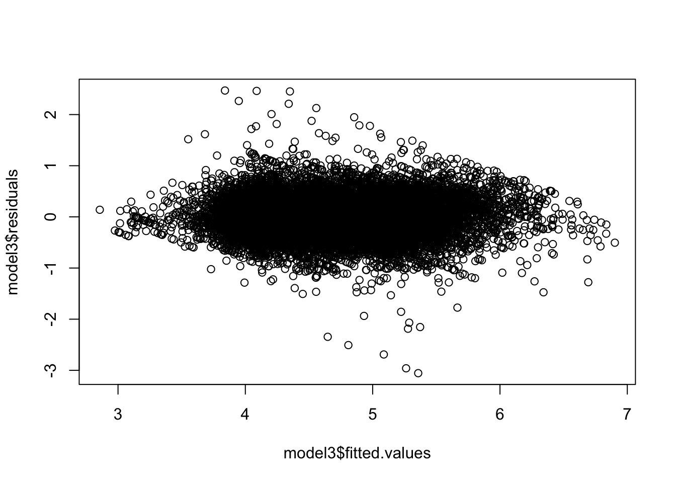
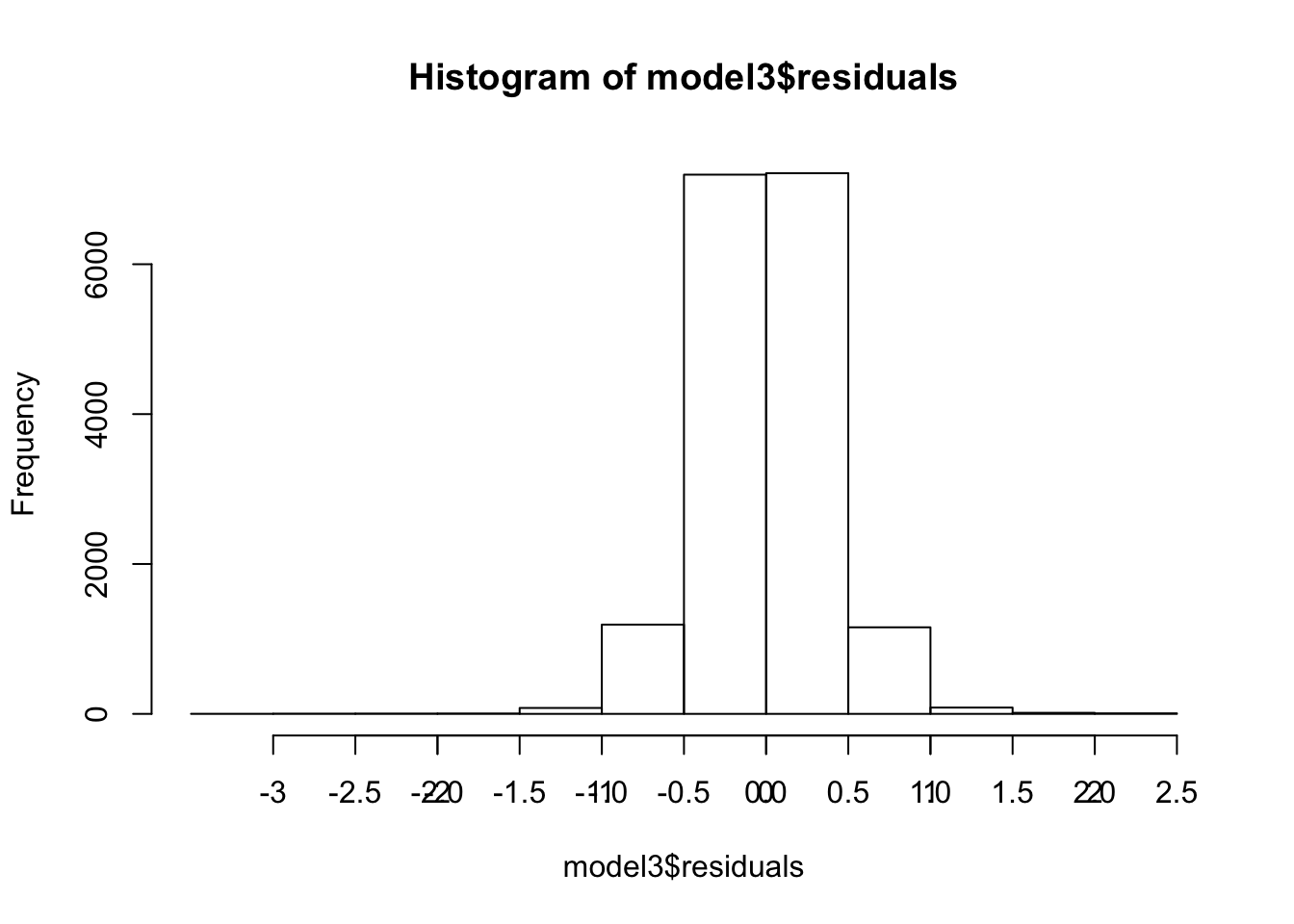
- Our residuals fit the requirements we would like to see which shows that our model is strong and we cannot really make this model significantly more accurate.
Now let’s input some sample data to test and see the expected value in price our model gives us.
- I created a data frame with my apartment’s information, and replaced all my NA values with .0000001, or almost 0. For example, I do not have a review score as I do not list on Airbnb, so I replaced that with almost 0. Same for my listings count. As for reviews, I inserted 1 since we take the log of this variable to normalize, and the log of 1 is equal to 0. I estimated that my listing will be available for 50% of the year and 50% of the month.
Jaggerslisting <- data.frame(accommodates=6, number_of_reviews=1
                             ,review_scores_rating=.0000001,availability_30=15
                             ,availability_365=182, bedrooms=1, beds=2
                             ,calculated_host_listings_count=.0000001,
                             bathrooms=1, neighbourhood_group_cleansed="Brooklyn",
                             room_type= "Entire home/apt" , host_identity_verified="t", cleaning_fee=50, guests_included= 6, property_type="Apartment",host_is_superhost="f")


JaggerslistingPrice <- predict(model3, newdata = Jaggerslisting)

#Since we log(price), we will need to take Exp(Of Our Result) to find our expected listing price per day per our model.

exp(JaggerslistingPrice)
## 1
## 100.5171- $100.5170614 as a listing price, not bad! Except I live in New York so if I hit the goal of 50% booking in the month, I will barely break even.
Lets predict with a 95% confidence interval with 5% level of sig. We can be 95% certain that the range of values will contain the true mean of the population.
##        fit      lwr      upr
## 1 100.5171 92.69864 108.9949- Since we are more focused on individual listings in our population, we can use the prediction interval. This will give us the range that we can be 95% certain the next value will fall between the intervals, and 5% will either fall under or over the intervals. We need to include uncertainty in the variation about our mean so this interval will be wider than our confidence interval.
predInterval <- predict(model3, newdata = Jaggerslisting, interval = "prediction", level = 0.95)
exp(predInterval)
## fit lwr upr
## 1 100.5171 48.94546 206.4273Please note that this is quite a bit wider than the confidence interval, indicating that the variation about the mean is fairly large. This means the datapoints of price are very spread out from the mean, indicating there is possibly more to the listing price than the variables used. I believe this ties into what I found in my research which was that commercial operators are saturating the Airbnb market, espeically in NYC.
Finally, Teaching the Machine to Learn Airbnb Prices
- Even with all the factors I have in my model, I expect a high RMSE due to the fact that Airbnb prices have been diluted to commercial operators. If not, then with about 13,600 (n * 0.80) observations in our training data, our model should be able to predict the price a little more accurately in our test data which will result in a LOW RMSE.
set.seed(99)
split <- sample.split(non0data$price, SplitRatio = 0.80)
train <- subset(non0data, split == 1)
test <- subset(non0data, split == 0)

predictTest <- predict(model3, type = "response", newdata=test)
dollar_predictTest <- exp(predictTest)
head(dollar_predictTest)
## 12 32 40 42 45 50
## 51.97977 82.90947 74.48427 227.43339 113.94938 293.66290rmse(test$price, dollar_predictTest)## [1] 67.43659The RMSE here is still high in my opinion after training the model with 13,600 observations. I would not seek a RMSE of 67.4365899 to efficiently price my property, and this is mostly because our model is getting trained to price property’s a bit low due to those commercial operators saturing the market with low price listings. I noticed that when the # of reviews increase, the price for the listing slightly decreases. This can either mean the model is not correct for this type of data, or that since commercial operators generally price very low they tend to have a lot of transactions which results in more reviews than the average lister.
#Conclusion These commercial operators are bringing down the prices of Airbnb listings and true home sharers cannot compete. In fact, 10% of these hosts (about 5,000) earned 48% of NYC’s total Airbnb revenue totaling $318 Million while the bottom 80% (over 40400) earned $209 Million in 2017. I believe once the playing field is leveled between consumer hosts and commercial hosts, the variance between individual fitted values and the population mean will start to decrease and the listing prices can be predicted with less noise.
